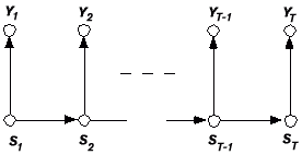
Figure 1 A graphical representation of the dependencies in a Hidden Markov Model.
A hidden Markov model (HMM) is a widely used probabilistic model for data that are observed in a sequential fashion (e.g., over time). A HMM makes two primary assumptions. The first assumption is that the observed data arise from a mixture of K probability distributions. The second assumption is that there is a discrete-time Markov chain with K states, which is generating the observed data by visiting the K distributions in Markov fashion. The "hidden" aspect of the model arises from the fact that the state-sequence is not directly observed. Instead, one must infer the state-sequence from a sequence of observed data using the probability model. Although the model is quite simple, it has been found to be very useful in a variety of sequential modeling problems, most notably in SPEECH RECOGNITION (Rabiner 1989) and more recently in other disciplines such as computational biology (Krogh et al. 1994). A key practical feature of the model is the fact that inference of the hidden state sequence given observed data can be performed in time linear in the length of the sequence. Furthermore, this lays the foundation for efficient estimation algorithms that can determine the parameters of the HMM from training data.
A HMM imposes a simple set of dependence relations between a sequence of discrete-valued state variables S and observed variables Y. The state sequence is usually assumed to be first-order Markov, governed by a K × K matrix of transition probabilities of the form p(St+1 = i | St+1 = j), that is, the conditional probability that the system will transit to state i at time t + 1 given that the system is in state j at time t (Markov 1913). The K probability distributions associated with each state, p(Yt | St = i), describe how the observed data Y are distributed given that the system is in state i. The transition probability matrix and the parameters of the K probability distributions are usually assumed not to vary over time. The independence relations in this model can be summarized by the simple graph in figure 1. Each state depends only on its predecessor, and each observable depends only on the current state. A large number of variations of this basic model exist, for example, constraints on the transition matrix to contain "null" transitions, generalizations of the first-order Markov dependence assumption, generalizations to allow the observations Yt to depend on past observations Yt-2, Yt-3, . . . , and different flexible parametrizations of the K probability distributions for the observable Ys (Poritz 1988; Rabiner 1989).
The application of HMMs to practical problems involves the solution of two related but distinct problems. The first is the inference problem, where one assumes that the parameters of the model are known and one is given an observed data sequence {Y1, . . . , YT}. How can one calculate p(Y1, . . . , YT | model), as in speech recognition (for example) when finding which word model, from a set of word models, explains the observed data best? Or how can one calculate the most likely sequence of hidden states to have generated {Y1, . . . , YT}, as in applications such as decoding error-correcting codes, where the goal is to determine which specific sequence of hidden states is most likely to have generated the data. Both questions can be answered in an exact and computationally efficiently manner by taking advantage of the independence structure of the HMM. Finding p(Y1, . . ., YT | model) can be solved by the forward-backward procedure, which, as the name implies, amounts to a forward pass through the possible hidden state sequences followed by a backward pass (Rabiner 1989). This procedure takes on the order of TK2 operations (linear in the length of the observed sequence). Similarly, the most likely sequence of hidden states for a given observation sequence can be found by the well-known Viterbi algorithm, which is a general application of DYNAMIC PROGRAMMING to this problem (Forney 1973). It also involves a forward and backward pass through the data and also takes order of TK2 operations.
Figure 1 A graphical representation of the dependencies in a Hidden Markov Model.
The second general problem to be solved in practice is that of estimation, that is, finding values for the HMM parameters; the K×K transition matrix, the parameters of the K observable probability distributions, and an initial probability distribution over the states. Implicit is the assumption that K is known (usually assumed to be the case in practice). Given K, the most widely used technique for estimation of HMM parameters is the Baum-Welch algorithm (Baum et al. 1970). The general idea behind the algorithm is as follows. Assume that the parameters are fixed at some tentative estimate. Use the forward-backward algorithm described earlier to infer the probabilities of all the possible transitions p(St+1 = j | St = i) between hidden states and all probabilities of observed data p(Yt | St = i), keeping the tentative parameters fixed. Now that one has estimates of the transitions and observation probabilities, it is possible to reestimate a new set of parameters in closed form. Remarkably, it can be shown that p(Y1, . . . , YT | θnew) ≥ p(Y1, . . . , YT | θold), that is, the likelihood of the new parameters is at least as great as that of the old, where θ denotes the particular HMM parameter set. Thus, iterative application of this two-step procedure of forward-backward calculations and parameter estimation yields an algorithm that climbs to a maximum of the likelihood function in parameter space. It turns out that this procedure is a special case of a general technique (known as the expectation-maximization or EM procedure; McLachlan and Krishnan 1997) for generating maximum-likelihood parameter estimates in the presence of hidden variables. Variations of the EM algorithm are widely used in machine learning and statistics for solving UNSUPERVISED LEARNING problems. The HMM parameter space can have many local maxima, making estimation nontrivial in practice. The Baum-Welch and EM procedures can also be generalized to maximum a posteriori and Bayesian estimation, where prior information and posterior uncertainty are explicitly modeled (e.g., Gauvain and Lee 1994).
It can be also be useful to look at HMMs from other viewpoints. For example, figure 1 can be interpreted as a simple Bayesian network and, thus, a HMM can be treated in complete generality as a particular member of the Bayesian network family (Smyth, Heckerman, and Jordan 1997). An advantage of this viewpoint is that it allows one to leverage the flexible inference and estimation techniques of BAYESIAN NETWORKS when investigating more flexible and general models in the HMM class, such as more complex sequential dependencies and multiple hidden chains.
Baum, L. E., T. Petrie, G. Soules, and N. Weiss. (1970). A maximization technique occurring in the statistical analysis of probabilistic functions of Markov chains. Ann. Math. Stat. 41:164-171.
Forney, G. D. (1973). The Viterbi algorithm. Proceedings of the IEEE 61:268-278.
Gauvain, J., and C. Lee. (1994). Maximum a posteriori estimation for multivariate Gaussian mixture observations of Markov chains. IEEE Trans. Sig. Audio Proc. 2:291-298.
Krogh, A., M. Brown, I. S. Mian, K. Sjolander, and D. Haussler. (1994). Hidden Markov models in computational biology: applications to protein modeling. J. Mol. Bio. 235:1501-1531.
Markov, A. A. (1913). An example of statistical investigation in the text of "Eugene Onyegin" illustrating coupling of "tests" in chains. Proc. Acad. Sci. St. Petersburg VI Ser. 7:153-162.
McLachlan, G. J., and T. Krishnan. (1997). The EM Algorithm and Extensions. New York: Wiley.
Poritz, A. M. (1988). Hidden Markov models: a guided tour. Proceedings of theIEEE International Conference on Acoustics, Speech and Signal Processing 1:7-13.
Rabiner, L. R. (1989). A tutorial on hidden Markov models and selected applications in speech recognition. Proceedings of the IEEE 77:257-285.
Smyth, P., D. Heckerman, and M. I. Jordan. (1997). Probabilistic independence networks for hidden Markov probability models. Neural Computation 9:227-269.
Elliott, R. J., L. Aggoun, and J. B. Moore. (1995). Hidden Markov Models: Estimation and Control. New York: Springer.
Huang, X. D., Y. Ariki, and M. A. Jack. (1990). Hidden Markov Models for Speech Recognition. Edinburgh: Edinburgh University Press.
MacDonald, I. L., and W. Zucchini. (1997). Hidden Markov and Other Models for Discrete-Valued Time Series. New York: Chapman and Hall.
![]() Copyright © 1999 Massachusetts Institute of Technology
Copyright © 1999 Massachusetts Institute of Technology