NEURAL NETWORKS are generally broken down into two broad categories: feedforward networks and recurrent networks. Roughly speaking, feedforward networks are net works without cycles (see PATTERN RECOGNITION AND FEEDFORWARD NETWORKS) and recurrent networks are networks with one or more cycles. The presence of cycles in a network leads naturally to an analysis of the network as a dynamic system, in which the state of the network at one moment in time depends on the state at the previous moment in time. In some cases, however, it is more natural to view the cycles as providing a specification of simultaneous constraints that the nodes of the network must satisfy, a point of view that need not involve any analysis of time-varying behavior. These two points of view can in principle be reconciled by thinking of the constraints as specifying the equilibrium states of a dynamic system.
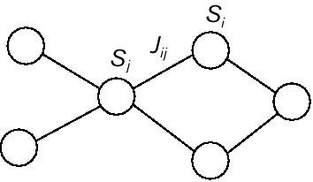
Let us begin by considering recurrent networks which admit an analysis in terms of equilibrium states. These networks, which include Hopfield networks and Boltzmann machines, are generally specified as undirected graphs, that is, graphs in which the presence of a connection from node Si to node Sj implies a connection from node Sj to node Si (see figure 1). The graph may be completely connected or partially connected; we will consider some of the implications associated with particular choices of connectivity later in the article.

Figure 1 A generic undirected recurrent network, in which the presence of a connection from node Si to node Sj implies a connection from node Sj to node Si. The value of the weight Jij is equal to Jji by assumption.
A Hopfield network is an undirected graph in which each node is binary (i.e., for each i, Si ∈ {-1, 1})., and each link is labeled with a real-valued weight Jij. Because the graph is undirected, Jij and Jji refer to the same link and thus are equal by assumption.
A Hopfield network also comes equipped with an energy function E, which can be viewed intuitively as a measure of the "consistency" of the nodes and the weights. The energy is defined as follows:

Equation 1
Consider, for example, the case in which Jij is positive. If Si and S j have the same value, then the energy is more negative (because of the minus sign), whereas if S i and Sj have opposite values, then the energy is more positive. The opposite statements hold when Jij is negative. Negative energy is "good," that is, it means that the nodes are more consistent with each other (with respect to the weights).
Let us define the "state" of the network to be an assignment of values to the nodes of the network. For Hopfield networks with N nodes this is simply a string of N bits.
Hopfield (1982) showed that the states of minimum energy are equilibrium states of a simple dynamic law known as the perceptron rule. In particular, suppose that at each moment in time a particular node i is chosen and that node updates its value as follows:

Equation 2
After a finite number of such updates the network will find itself in a state that is a local minimum of the energy E and it will no longer move from that state.
Hopfield networks can be utilized to perform a number of information-processing tasks. One such task is that of CONSTRAINT SATISFACTION. Here the weights Jij are set, either by design or via a learning algorithm (see MACHINE LEARNING), to encode a particular set of desired constraints between nodes. Minimizing the energy corresponds to finding a state in which as many of the constraints are met as possible. Another task is associative memory, in which the minima of the energy function are viewed as memories to be retrieved. The updating of the system according to Eq. (2) corresponds to the "cleaning up" of corrupted memories. Finally, Hopfield networks can be used for optimization applications; in such applications the weights are chosen by design so that the energy E is equal to the quantity that it is desired to optimize.
The formulation of the Hopfield model in the early 1980s was followed by the development of the Boltzmann machine (Hinton and Sejnowski 1986), which is essentially a probabilistic version of the Hopfield network. The move to probabilities has turned out to be significant; it has led to the development of new algorithms for UNSUPERVISED LEARNING and SUPERVISED LEARNING, and to more efficient algorithms for Hopfield networks.
A Boltzmann machine is characterized by a probability distribution across the states of a Hopfield network. This distribution, known as the Boltzmann distribution, is the exponential of the negative of the energy of the state:

Equation 3
where Z is a normalizing constant (the sum across all states of the numerator), and T is a scaling constant. The Boltzmann distribution gives higher probability to states with lower energy, but does not rule out states with high energy. As T goes to zero, the lower energy states become the only ones with significant probability and the Boltzmann machine reduces to a Hopfield network.
There are three basic methods that have been used for calculating probabilities for Boltzmann machines: exact calculation, Monte Carlo simulation, and mean field methods.
Exact calculation methods are generally based on recursive procedures for transforming or eliminating nodes. One such method, known as decimation, is based on the fact that it is possible to remove, or "decimate," a node lying between a pair of other nodes, replacing the removed node with its weights by a single "effective" weight, while maintaining the same marginal probability on the remaining pair of nodes (Saul and Jordan 1994). For graphs with a chain-like or tree-like connectivity pattern, this procedure can be applied recursively to provide a general method for calculating probabilities under the Boltzmann distribution. There are interesting links between this procedure and exact algorithms for HIDDEN MARKOV MODELS and other more general probabilistic graphs known as BAYESIAN NETWORKS (Lauritzen 1996).
Monte Carlo simulation implements a stochastic search among states, biasing the search toward states of high probability (see also GREEDY LOCAL SEARCH). One simple Monte Carlo procedure is known as "Gibbs sampling" (Geman and Geman 1984). It turns out that Gibbs sampling for the Boltzmann machine is equivalent to the use of the perceptron rule [Eq. (2)] with a noisy threshold. Gibbs sampling was the method proposed in the original paper on the Boltzmann machine (Hinton and Sejnowski 1986). To speed the search, Hinton and Sejnowski also proposed the use of "simulated annealing," in which the temperature T is started at a high value and gradually decreased.
Finally, mean field methods take advantage of the fact that in networks that have dense connectivity each node has a value (under the Boltzmann distribution) that is well determined by its neighbors (by the law of large numbers). Thus it is possible to find and to exploit approximate deterministic constraints between nodes. The resulting equations of constraint, known as "mean field equations," generally turn out to once again have the form of the perceptron update rule, although the sharp decision of Eq. (2) is replaced with a smoother nonlinear function (Peterson and Anderson 1987).
Mean field methods can also be utilized with decreasing T. If T is decreased to zero, this idea, referred to as "deterministic annealing," can be applied to the Hopfield network. In fact deterministic annealing has become the method of choice for the update of Hopfield networks, replacing the simple dynamics of Eq. (2).
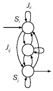
General recurrent networks are usually specified by drawing a directed graph (see figure 2). In such graphs, arbitrary connectivity patterns are allowed; that is, there is no requirement that nodes are connected reciprocally. We associate a real-valued weightJij with the link from node j to node i, letting J ij equal zero if there is no link.

Figure 2 A generic recurrent network. The presence of cycles in the graph distinguishes these networks from the class of feedforward networks. Note that there is no requirement of reciprocity as in the Hopfield or Boltzmann networks.
At time t, the ith node in the network has an activation value Si[t], which can either be a discrete value or a continuous value. Generally the focus is on discrete-time systems (see also AUTOMATA), in which t is a discrete index, although continuous-time systems are also studied (see also CONTROL THEORY). The update rule defining the dynamics of the network is typically of the following form:

Equation 4
where the function f is generally taken to be a smooth nonlinear function.
General recurrent networks can show complex patterns of dynamic behavior (including limit cycles and chaotic patterns), and it is difficult to place conditions on the weights Jij that guarantee particular kinds of desired behavior. Thus, researchers interested in time-varying behavior of recurrent networks have generally utilized learning algorithms as a method of "programming" the network by providing examples of desired behavior (Giles, Kuhn, and Williams1994).
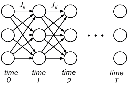
A general purpose learning algorithm for recurrent networks, known as backpropagation-in-time, can be obtained by a construction that "unrolls" the recurrent network (Rumelhart et al. 1986). The unrolled network has T + 1 layers of N nodes each, obtained by copying the N of the recurrent network at every time step from t = 0 to t = T (see figure 3). The connections in the unrolled network are feedforward connections that are copies of the recurrent connections in the original network. The result is an unrolled network that is a standard feedforward network. Applying the standard algorithm for feedforward networks, in particular backpropagation, yields the backpropagation-in-time algorithm.

Figure 3 An "unrolled" recurrent network. The nodes Si in the recurrent network in Figure 2 are copied in each of T + 1 time slices. These copies represent the time-varying activations Si[t]. The weights in each slice are time-invariant; they are copies of the corresponding weights in the original network. Thus, for example, the weights between the topmost nodes in each slice are all equal to Jii, the value of the weight from unit Si to itself in the original network.
Backpropagation-in-time and similar algorithms have a general difficulty in training networks to hold information over lengthy time intervals (Bengio, Simard, and Frasconi 1994). Essentially, gradient-based methods utilize the derivative of the state transition function of the dynamic system, and for systems that are able to hold information over lengthy intervals this derivative tends rapidly to zero. Many new ideas in recurrent network research, including the use of embedded memories and particular forms of prior knowledge, have arisen as researchers have tried to combat this problem (Frasconi et al. 1995; Omlin and Giles 1996).
Finally, there has been substantial work on the use of recurrent networks to represent finite automata and the problem of learning regular languages (Giles et al. 1992).
Bengio, Y., P. Simard, and P. Frasconi. (1994). Learning long-term dependencies with gradient descent is difficult. IEEE Transactions on Neural Networks 5:157-166.
Frasconi, P., M. Gori, M. Maggini, and G. Soda. (1995). Unified integration of explicit rules and learning by example in recurrent networks. IEEE Transactions on Knowledge and Data Engineering 7:340-346.
Geman, S., and D. Geman. (1984). Stochastic relaxation, Gibbs distributions, and the Bayesian restoration of images. IEEE Transactions on Pattern Analysis and Machine Intelligence 6:721-741.
Giles, C. L., G. M. Kuhn, and R. J. Williams. (1994). Dynamic recurrent neural networks: Theory and applications. IEEE Transactions on Neural Networks 5:153-156.
Giles, C. L., C. B. Miller, D. Chen, H. H. Chen, G. Z. Sun, and Y. L. C. Lee. (1992). Learning and extracting finite state automata with second-order recurrent neural networks. Neural Computation 4:393-401.
Hinton, G. E., and T. Sejnowski. (1986). Learning and relearning in Boltzmann machines. In D. E. Rumelhart and J. L. McClelland, Eds., Parallel Distributed Processing, vol. 1. Cambridge, MA: MIT Press, pp. 282-317.
Hopfield, J. J. (1982). Neural networks and physical systems with emergent collective computational abilities. Proceedings of the National Academy of Sciences 79:2554-2558.
Lauritzen, S. L. (1996). Graphical Models. Oxford: Oxford University Press.
Omlin, C. W., and C. L. Giles. (1996). Extraction of rules from discrete-time recurrent neural networks. Neural Networks 9:41-79.
Peterson, C., and J. R. Anderson. (1987). A mean field theory learning algorithm for neural networks. Complex Systems 1:995-1019.
Rumelhart, D. E., G. E. Hinton, and R. J. Williams. (1986). Learning internal representations by error propagation. In D. E. Rumelhart and J. L. McClelland, Eds., Parallel Distributed Processing, vol. 1. Cambridge, MA: MIT Press.
Saul, L. K., and M. I. Jordan. (1994). Learning in Boltzmann trees. Neural Computation 6:1174-1184.
Amit, D. (1989). Modelling Brain Function. Cambridge: Cambridge University Press.
Cohen, M., and S. Grossberg. (1983). Absolute stability of global pattern formation and parallel memory storage by competitive neural networks. IEEE Transactions on Systems, Man, and Cybernetics 13:815-826.
Elman, J. (1990). Finding structure in time. Cognitive Science 14:179-211.
Haykin, S. (1994). Neural Networks: A Comprehensive Foundation. New York: Macmillan.
Hertz, J., A. Krogh, and R. G. Palmer. (1991). Introduction to the Theory of Neural Computation. Redwood City, CA: Addison-Wesley.
Jensen, F. (1996). An Introduction to Bayesian Networks. London: UCL Press (also published by Springer-Verlag).
Jordan, M. I. (1997). Serial order: A parallel, distributed processing approach. In J. W. Donahoe and V. P. Dorsel, Eds., Neural Network Models of Cognition: A Biobehavioral Approach. Amsterdam: Elsevier.
Jordan, M. I., and C. Bishop. (1997). Neural networks. In A. B. Tucker, Ed., CRC Handbook of Computer Science. Boca Raton, FL: CRC Press.
Jordan, M. I., and D. E. Rumelhart. (1992). Forward models: Supervised learning with a distal teacher. Cognitive Science 16:307-354.
Lang, K. J., A. H. Waibel, and G. E. Hinton. (1990). A time-delay neural network architecture for isolated word recognition. Neural Networks 3:23-43.
Mozer, M. C. (1994). Neural net architectures for temporal sequence processing. In A. S. Weigend and N. A. Gershenfeld, Eds., Time Series Prediction. Redwood City, CA: Addison-Wesley, pp. 243-264.
Pearlmutter, B. A. (1989). Learning state space trajectories in recurrent neural networks. Neural Computation 1:263-269.
Rabiner, L. R. (1989). A tutorial on Hidden Markov models and selected applications in speech recognition. Proceedings of the IEEE 77:257-286.
Schmidhuber, J. (1992). Learning complex, extended sequences using the principle of history compression. Neural Computation 4:234-242.
Smyth, P., D. Heckerman, and M. I. Jordan. (Forthcoming). Probabilistic independence networks for hidden Markov probability models. Neural Computation to appear.
Tsoi, A. C., and A. Back. (1994). Locally recurrent globally feedforward networks: A critical review of architectures. IEEE Transactions on Neural Networks 5:229-239.
Williams, R. J. (1989). A learning algorithm for continually running fully recurrent neural networks. Neural Computation 1:270-280.